Geographical Information System (QGIS) Tutorial: Module 1

By the end of this module, you should be able to: 

• Navigate QGIS’s user interface (UI) and locate commonly used tools and functions.
• Load vector shapefiles, raster images from various sources. 
• Create and import data into geopackages (gpkg). 
• Define and transform data projections/coordinate systems.
• Understand how attribute tables store and structure data in GIS.
• Load and change base maps online using QGIS. 
• Understand the difference between “data file”, “layer”, “layout”, and “map document”.

Before you start the exercise below, please make sure you have installed the long-term release (LTR) version of the QGIS. At the time of preparing this document, the LTR is v3.28. 

Download the installation package here. QGIS is an open source software, compatible with both Windows and Mac. 

Requirements

• A laptop (PC or Mac). If you do not have one, please loan one from CADlab (30 days maximum).  
• QGIS Long-Term Release version (the current LTR is QGIS 3.28 at the time of preparing this document). Download here.
• M1 input files

Resources

• QGIS 30 minute introduction (YouTube video)
• QGIS 70 minute overview (YouTube video) 
• QGIS self-guided study (qgistutorials.com)

Legend:
[Action]
! Important notes from the instructor !

In this section, we will first explore the QGIS user interface (UI) so that you are familiar with the menu options, toolbars, map canvas and layers list that form the basic structure of the interface. 

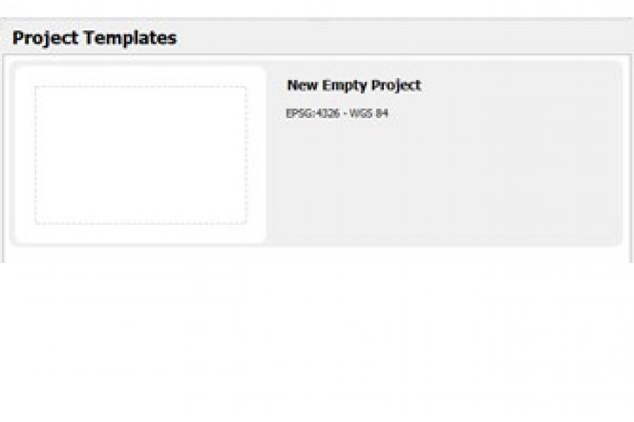
You will be greeted with the interface shown below. 

1. Layers list 
2. Toolbars
3. Map canvas 
4. Browser (to access local and online data)
5. Processing toolbox 
6. Current “on-the-fly” map scale and projection/coordinate system 

If you prefer a dark themed QGIS UI, you can switch to Night Mapping mode: [Settings -> Options -> General -> UI Theme]. You will have to [restart QGIS] to see the change. 

Next, let’s load some data onto the map canvas! 
Please [download the file from the corresponding folder]. [Save the file on your Desktop] (for now). QGIS will not be able to read zipped/compressed files. !Please avoid loading data from a network drive (e.g., OneDrive or Dropbox)! It will cause delays and generally is not a good habit to develop. 
You will need to unzip the file you have just downloaded. 
Windows: [Right click the file -> Extract] 
Mac: [double click the file]
You can now [delete the zipped/compressed file]

To turn on / off each layer, you can [check / uncheck the box] on the left side of the layer name under the Layers pane. You can also change the drawing order simply by dragging the layer up and down under the Layers pane.   

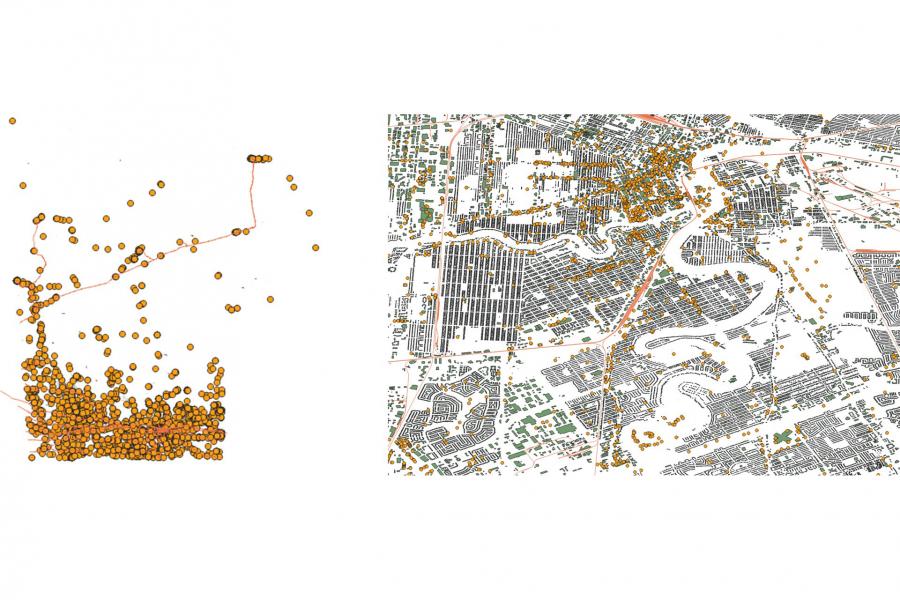
It is not the prettiest map to look at when zooming out (screenshot, left). It gets a bit better when zooming in (screenshot, right). We will worry about the styling (or map symbology in GIS lingo) later. For now we will be sticking with the default symbology settings from QGIS.  

You might want to save this QGIS Project before moving to the next step. 
[Cltr + S] (Windows) or [Cmd + S] (Mac) 

In some cases, you might find yourself downloading data in formats other than .shp. Do not worry. QGIS can read most common geospatial data formats, such as json, kml (Google Earth), geodatabase (.gdb, native to ArcGIS, another common software used in the GIS community), geopackage (.gpkg, native to QGIS), and even Excel tables (.csv) with coordinates information. 

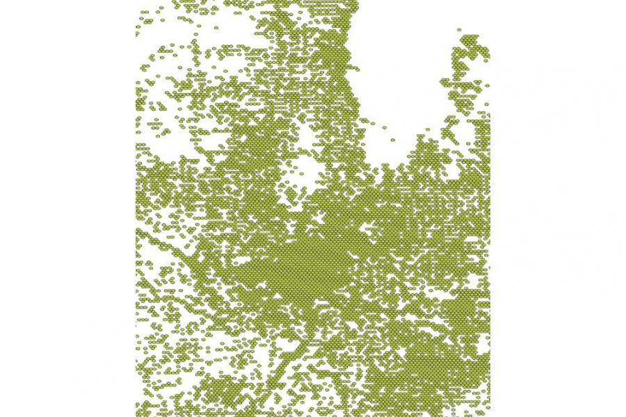
In the same folder, you will notice another file, kontur_population_CA_20231101.gpkg. This is a geopackage file containing a congregation of hexagons, each of which contains a population count value. The data is sourced from the Humanitarian Data Exchange (HDX, download here). The data you have is for Canada. 

Raster (or raster image) is another way to represent geographic data. A raster image typically consists of connected pixels (short for picture elements), each of which contains a value. Almost all satellite images nowadays are stored digitally as rasters (before it was in analogue films). 

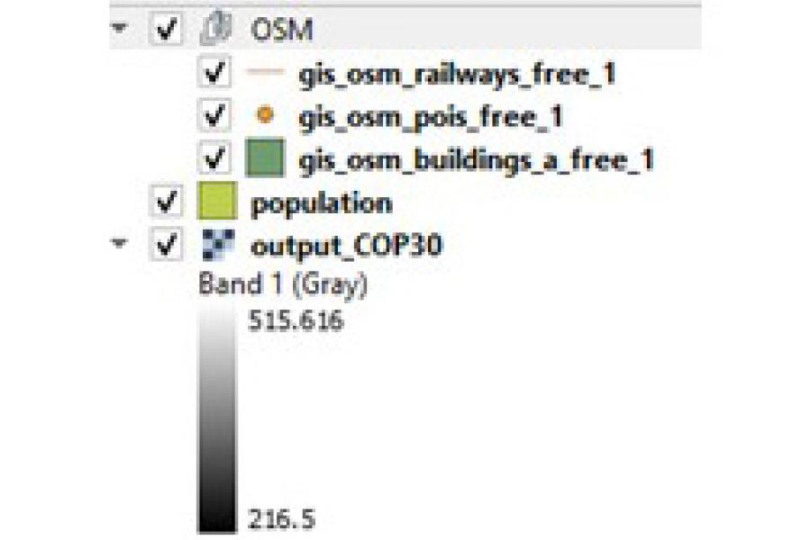
Terrain information is also typically stored as rasters with each pixel containing a value representing the elevation (usually in meters). This is known as a digital terrain model (DTM). In the folder, you will find a DTM raster for a part of southern Manitoba: output_COP30.tiff. This raster was sourced from https://portal.opentopography.org/datasets and it is free to use! 

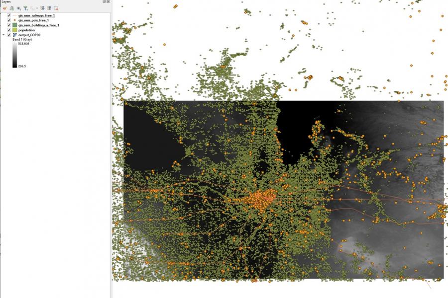
My QGIS window now looks like the screenshot above -- What a mess.
Like many Adobe applications that you might be more comfortable with, QGIS also allows you to group layers and give it a meaningful name. 

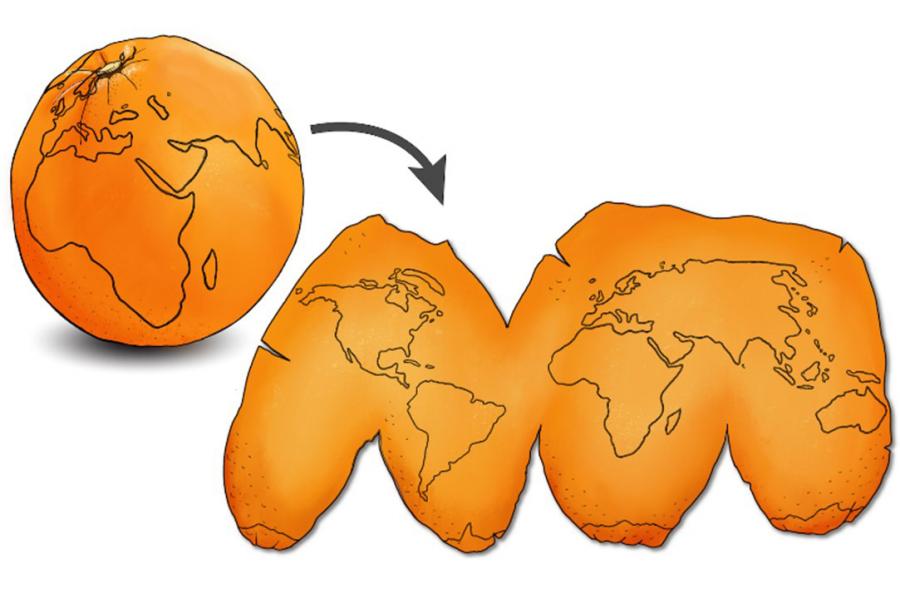
The best way to represent the Earth is to use a three-dimensional (3D) model. But for practical reasons, most maps are created for two-dimensional (2D) devices (e.g., paper, screens etc.). Inevitabley, when presenting a 3D sphere (like an orange) onto a 2D surface (after you peel the orange), there will be distortions particularly of its shape, size, and direction.

! The process of this 3D-to-2D mathematical transformation is a map projection !

!All maps come with distortions! But some are more suitable than others (or more accurately speaking, tolerable) for certain applications and scales. For example, Google Maps uses a Mercator projection which largely distorts the size of many countries, and the farther away you are from the Equator, the more distorted the map becomes! 

Fun fact: Do you know that Africa is 14 times bigger than Greenland? 

And have you noticed that most 2D world maps are always Euro-centric: the Pacific Ocean always splits in half while the Atlantic Ocean and the European continent are centred and in one piece? Indeed, maps are also political, but this is a topic for another day! 

QGIS allows us to !manipulate projection of the map canvas “on-the-fly” as well as the spatial data! (vector and raster). For local mapping projects, the Universal Transverse Mercator coordinate system (UTM) is commonly used. Winnipeg is in UTM Zone 14 North, with a EPSG code of 32610. (EPSG code is a fast way to find the projection you need in mapping software such as QGIS). 

By default, a new QGIS project will open with a geographic coordinate system (EPSG 4326). UTM is also a preferred projection in many applications because it measures distances in linear unit (meters) while geographic coordinate systems use decimal degrees (latitude and longitude). In the following steps, we will transform the projections of all the layers we have imported so far to UTM 14 North. 

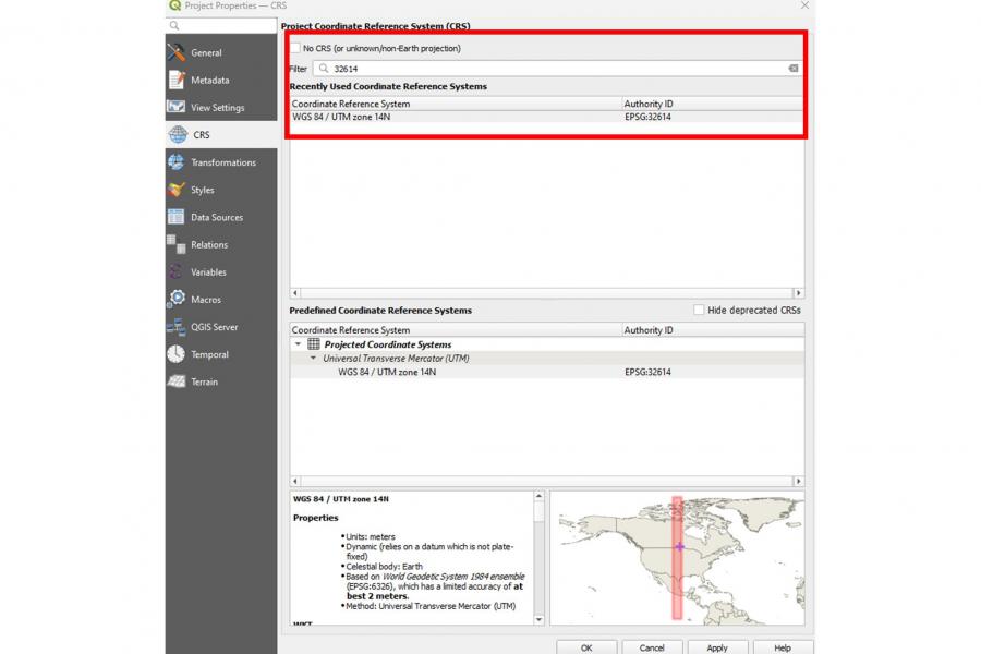
[Click EPSG: 4326] at the lower right corner of the QGIS interface. A new window will pop out where you can change the map canvas projection. Again, this does not change the projection of the actual data! 
[Type 32614 in Filter -> Entre -> Double click WGS 84 / UTM zone 14N]
You will know this is the right zone because QGIS shows regions (red bar on the world map) covered by UTM 14N and Winnipeg is inside (the purple cross). Obviously if you are mapping for other regions in Canada, you will need a different zone (Canada covers 22 zones, from UTM 7N to 22N). See screenshot below.
[Click Apply] 
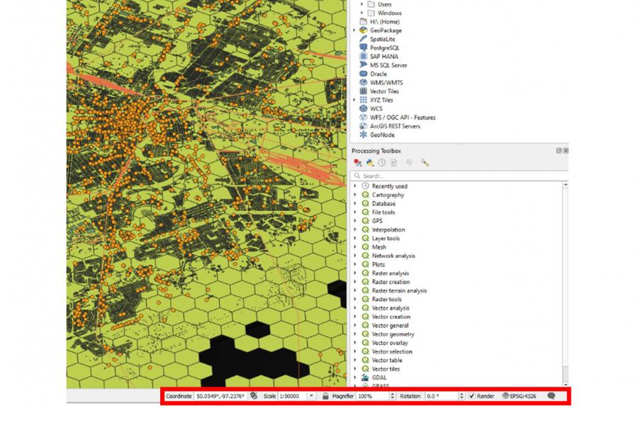
DO NOT zoom in or out. Do you notice how the scale has changed, even though it is still around Winnipeg. The location is now also determined using a UTM system with a unit of meters. !Scale is determined by the projection and in which unit locations are being measured! 

Also, hey! Our hexagons look a bit different now! Looks at these train tracks!

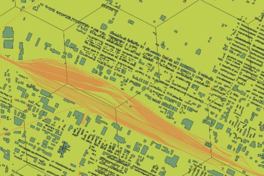
Alternatively, we could also change the projection of the actual data, but it is beyond the scope of this lab. You will learn more about them throughout the studio or in my digital mapping course.

That was intense? We will have some fun with QGIS in the last section. 
Base map is of popular demand in your design work, especially when you cannot physically visit the site. QGIS offers many base maps options, and you can stream it directly from the web (like Netflix but for base maps!). 

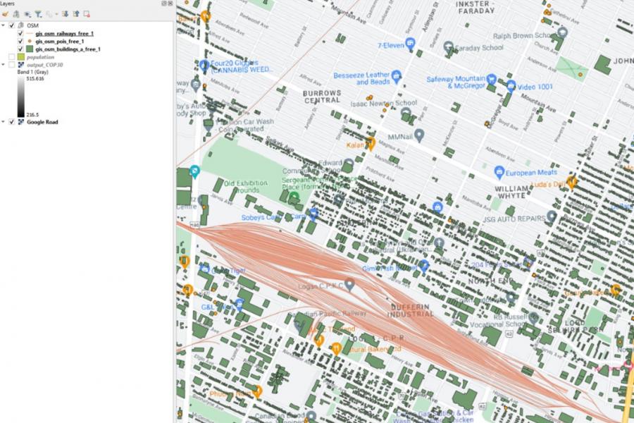
To load the base map, you can either double click the map you like or drag-and-drop it to the map canvas. Make sure base map is on the bottom of the Layers list.
I loaded the Google Road and turned off my hexagon layer so we can see the base map. 

Let’s add more base map to the XYZ tile list in your QGIS. You will only need to do it once as long as you do not uninstall QGIS. 
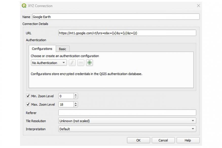
[XYZ Tiles -> Right click -> New Connection] (This allows QGIS to add open-source base maps directly. If you are working on your personal computer, please make sure you have access to Internet). Here is a list of more URLs if you are interested in other types/styles of base maps. 
[Replace the Name and URL in the XYZ Connection window] (screenshot) with the list below. Leave all the other parameters as it is. 

• OpenTopoMap: https://tile.opentopomap.org/{z}/{x}/{y}.png 
• OpenStreetMap: http://tile.openstreetmap.org/{z}/{x}/{y}.png 
• Google Hybrid: https://mt1.google.com/vt/lyrs=y&x={x}&y={y}&z={z} 
• Bing Aerial: http://ecn.t3.tiles.virtualearth.net/tiles/a{q}.jpeg?g=1 

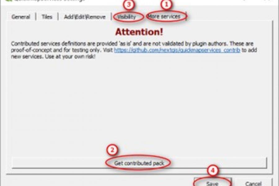
Impressed yet? Let’s add a few more! Please follow the steps outlined below. 

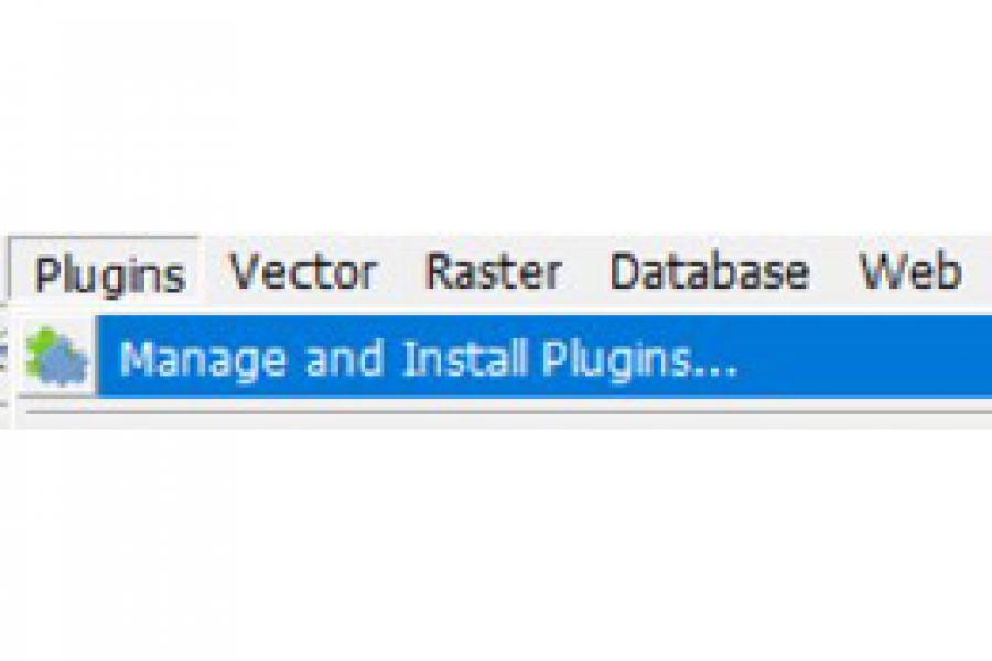
Since QGIS is an open-source software, it also allows users (like you and me) to create and upload plug-ins. Plug-ins are extensions of existing tools offered by QGIS’ built-in functions. It is often made by the people and for the people! 

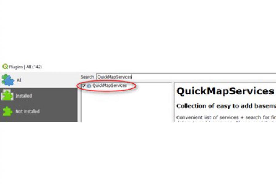
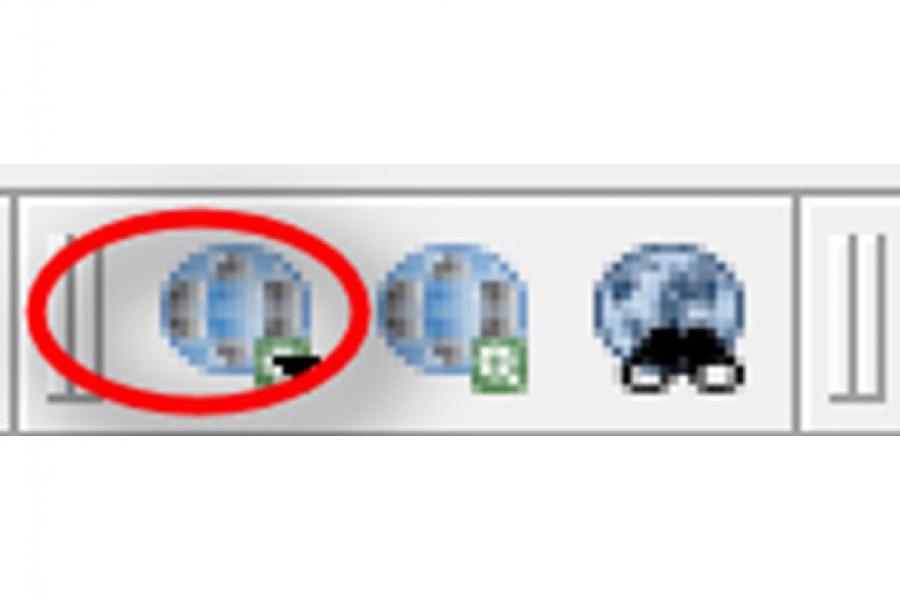
We will be installing a plug-in called QuickMapServices that allows you to access an extensive list of base maps offered by Google, NASA, OpenStreetMaps, and many others. It is of course completely free. 

The end!